A Beginner's Guide to TypiClust

How to pick the right samples to label when your labelling budget is small.

This is my very first blog post ever, so please be forgiving. My goal here is simple: walk you through TypiClust, an active learning algorithm from the paper "Active Learning on a Budget: Opposite Strategies Suit High and Low Budgets" (Hacohen et al., 2022), in a way that makes sense even if you've never heard of active learning before. By the end of this post, you'll understand:

1. What active learning is, and why the usual approaches quietly break when you don't have a lot of money (i.e. resources).
2. The core intuition behind TypiClust.
3. How to implement it yourself, step by step, in a Python notebook.

All the code is available on GitHub, and I've also written a more academic report (also on GitHub) if you want to dig deeper into the theory.

A Quick Primer: What is Active Learning?

Imagine you're training a cat-vs-dog classifier and you have one million unlabelled images, but only enough budget to hire a human to label 200 of them. Which 200 do you pick?

Picking randomly feels wasteful — most images look almost the same. What you really want is to pick the images that will teach the model the most.

That is exactly what active learning is for: the method of choosing which data points to label next. The standard loop looks like this:

1. Train a model on whatever labels you already have.
2. Use the model to score every unlabelled sample (e.g. "how unsure am I about this one?").
3. Send the top-scoring samples off to a human labeller.
4. Add the newly labelled samples to your training set.
5. Repeat until you're out of budget.

Most classical active learning methods — for example Margin Sampling or BADGE — follow this loop and rely on the model's own uncertainty to pick samples. And for a long time, the community assumed: more clever uncertainty → better results. Simple.

Well — not exactly.

The Problem: Classical Active Learning Quietly Breaks on Small Budgets

Here is where the TypiClust paper drops a surprising result.

The authors show, both theoretically and empirically, that in low-budget settings classical active learning methods often perform worse than random sampling.

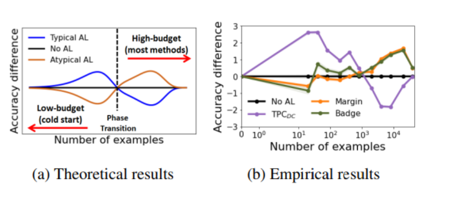
The intuition is that uncertainty-based methods love to pick hard, outlier-ish points — samples near the decision boundary where the model is confused. And at the start of training, when the model barely knows anything, those "hard" points are often too hard. They're noisy, weird, or just unrepresentative. Labelling them teaches the model very little about the data in general.

There's an inflection point: once you already have enough labels to understand the "easy majority" of the data, then picking hard boundary cases starts to help. Before that? Don't.

The authors call this the opposite-strategy phenomenon: what's best in a high-budget regime is often the worst in a low-budget regime.

So — what should we do when the budget is tight?

The Core Idea of TypiClust

In a low-budget regime, we want our first labels to be representative — points that look like a lot of other points. If we label one "very typical" cat picture, we've effectively taught the model what a cat generally looks like. Labelling the weird outlier cat in a mask? Much less bang for your buck.

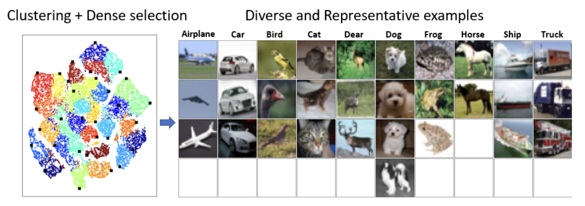
Formally, TypiClust boils down to three steps:

1. Cluster the feature space (a vector representation of your data that's easily digestible for the model) into groups of similar-looking samples.
2. Prioritise clusters that don't already have many labels in them.
3. Within each chosen cluster, pick the most typical sample — the one sitting deepest inside a dense crowd of neighbours.

Measuring Typicality

So what is "typicality"? The paper defines it as:

Don't worry about the scary notation — the idea is quite simple:

• For each sample x, find its K nearest neighbours in feature space.
• Compute the average distance from x to those neighbours.
• Take the inverse of that average distance.

If the average distance to your neighbours is small, you're surrounded by lookalikes → you're very typical → high score. If the average distance is large, you're floating off alone in feature space → you're an outlier → low score.

That's it. Outliers get low typicality, inliers get high typicality.

Here's the Python implementation, using FAISS to make the nearest-neighbour search fast:

import faiss
import numpy as np

def get_typicality(features: np.ndarray, num_neighbors: int) -> np.ndarray:
    """Return a typicality score for each feature vector.

    Typicality = 1 / (mean distance to K nearest neighbours).
    High score => point sits in a dense region.
    """
    if num_neighbors < 1:
        raise ValueError(f"num_neighbors must be at least 1, got {num_neighbors}")

    features = features.astype(np.float32)
    d = features.shape[1]

    # Use GPU FAISS if available, otherwise fall back to CPU.
    index = faiss.IndexFlatL2(d)
    try:
        index = faiss.index_cpu_to_all_gpus(index)
    except Exception:
        pass  # no GPU FAISS — CPU is fine, just slower

    index.add(features)

    # Search for K+1 neighbours because the closest one is always
    # the point itself (distance 0). We throw that one away.
    distances, _ = index.search(features, num_neighbors + 1)
    mean_distance = distances[:, 1:].mean(axis=1)

    # Add a tiny epsilon to avoid division by zero for duplicate points.
    return 1.0 / (mean_distance + 1e-5)

Two Things You Need Before You Can Run TypiClust

Before we can actually run TypiClust on a dataset, we need two ingredients. These aren't part of the algorithm itself, but the whole method is built on top of them.

1 — A feature map

TypiClust measures distances between samples — but distance in what space? Not in pixel space, because two images of the same cat from slightly different angles are miles apart in raw pixels.

So we feed every image in our dataset through an encoder network — typically a self-supervised model like SimCLR, DINO, or even the convolutional backbone of whatever classifier you're training — and collect the resulting feature vectors.

import torch
from torch.utils.data import DataLoader

def extract_features(model, dataloader, device):
    """Push every image through the encoder and collect the embeddings."""
    model.eval()
    all_features = []
    with torch.inference_mode():
        for images, _ in dataloader:
            images = images.to(device)
            features = model(images)
            all_features.append(features.cpu().numpy())
    return np.concatenate(all_features, axis=0)

2 — A clustering of the data

TypiClust assumes we've split the feature space into clusters — groups of samples that sit close together. The original paper uses K-Means because it's simple, fast, and works surprisingly well on top of good embeddings.

from sklearn.cluster import KMeans, MiniBatchKMeans

def cluster_with_kmeans(features: np.ndarray, num_clusters: int) -> np.ndarray:
    if num_clusters <= 50:
        model = KMeans(n_clusters=num_clusters)
    else:
        # MiniBatch is dramatically faster for large K, with a tiny quality hit.
        model = MiniBatchKMeans(n_clusters=num_clusters, batch_size=5000)
    model.fit(features)
    return model.labels_

The Selection Strategy

Now we have features and clusters. Time to actually pick samples.

TypiClust walks through the clusters in a specific order and picks the most typical point from each, one at a time, round-robin style:

1. Rank clusters — those with the fewest labels so far go first; ties are broken by cluster size (bigger clusters first, because they represent more of the data).
2. Loop through clusters, and from each cluster's unlabelled points, pick the one with the highest typicality.
3. Mark it as labelled, move to the next cluster.
4. When you've cycled through every cluster, start again from the top until you hit your budget.

This balances two pressures: coverage (hit every region of the data) and quality (always pick the most representative point in that region).

def typiclust(features, labeled_idx, unlabeled_idx, budget,
              min_cluster_size=5, k_nn=20):
    """
    Pick `budget` samples from `unlabeled_idx` using TypiClust.
    Returns (newly_selected, remaining_unlabeled).
    """
    # 1. Cluster the full feature space.
    num_clusters = min(len(labeled_idx) + budget, 500)
    Cls = KMeans if num_clusters <= 50 else MiniBatchKMeans
    cluster_labels = Cls(n_clusters=num_clusters, random_state=0).fit_predict(features)

    # 2. Build a local view of labelled + unlabelled points.
    all_idx = np.concatenate([labeled_idx, unlabeled_idx])
    feats   = features[all_idx]
    labels  = cluster_labels[all_idx]
    n_lab   = len(labeled_idx)
    available = np.zeros(len(all_idx), dtype=bool)
    available[n_lab:] = True   # only unlabelled points are selectable

    # 3. Rank clusters: fewest existing labels first, then biggest first.
    cluster_ids, cluster_sizes = np.unique(labels, return_counts=True)
    lab_counts = {cid: int((labels[:n_lab] == cid).sum()) for cid in cluster_ids}
    cluster_order = sorted(
        [(cid, sz, lab_counts[cid])
         for cid, sz in zip(cluster_ids, cluster_sizes) if sz > min_cluster_size],
        key=lambda x: (x[2], -x[1])   # (existing_count ASC, size DESC)
    )
    cluster_order = [row[0] for row in cluster_order]

    # 4. Round-robin: one pick per cluster per pass.
    selected, ptr = [], 0
    while len(selected) < budget:
        if ptr >= len(cluster_order):
            ptr = 0
        cluster = cluster_order[ptr]; ptr += 1

        candidates = np.where((labels == cluster) & available)[0]
        if len(candidates) == 0:
            if not np.any(np.isin(labels[available], cluster_order)):
                break   # pool exhausted
            continue

        scores = get_typicality(feats[candidates], num_neighbors=k_nn)
        best   = candidates[scores.argmax()]
        selected.append(best)
        available[best] = False

    # 5. Map local indices back to dataset indices.
    active_set = all_idx[np.array(selected)]
    remaining  = np.setdiff1d(unlabeled_idx, active_set)
    return active_set, remaining

That's the whole algorithm. Once you've absorbed the three-step recipe — cluster, prioritise, pick typical — everything else is plumbing.

Putting It All Together: A Minimal Active Learning Loop

Here is a small, self-contained training script on CIFAR-10. This is stripped down for clarity — the full, experiment-ready version is in the repository.

SEED        = 42
NUM_SAMPLES = 1000      # a subset of CIFAR-10 so runs stay fast

LSET_RATIO = 0.1        # 10% seed labels
USET_RATIO = 0.8        # 80% unlabelled pool
VAL_RATIO  = 0.1        # 10% validation

BATCH_SIZE         = 128
LR                 = 1e-3
EPOCHS_PER_EPISODE = 5
NUM_EPISODES       = 5     # active learning rounds
BUDGET             = 50    # new labels per round

import random, numpy as np, torch

def set_seed(seed):
    random.seed(seed); np.random.seed(seed)
    torch.manual_seed(seed); torch.cuda.manual_seed_all(seed)
    torch.backends.cudnn.deterministic = True
    torch.backends.cudnn.benchmark     = False

set_seed(SEED)
device = torch.device("cuda" if torch.cuda.is_available() else "cpu")

import torch.nn as nn

class SmallCNN(nn.Module):
    def __init__(self, num_classes=10):
        super().__init__()
        self.features = nn.Sequential(
            nn.Conv2d(3, 16, 3, padding=1), nn.ReLU(inplace=True), nn.MaxPool2d(2),
            nn.Conv2d(16, 32, 3, padding=1), nn.ReLU(inplace=True), nn.MaxPool2d(2),
        )
        self.classifier = nn.Sequential(
            nn.Flatten(),
            nn.Linear(32 * 8 * 8, 64), nn.ReLU(inplace=True),
            nn.Linear(64, num_classes),
        )

    def forward(self, x):
        return self.classifier(self.features(x))

history = []
for episode in range(NUM_EPISODES):
    print(f"\n= Episode {episode+1}/{NUM_EPISODES} "
          f"| labeled={len(lSet)} | unlabeled={len(uSet)} =")

    # 1. Train on the current labelled set.
    train_loader = make_train_loader(full_dataset, lSet, train_transform, SEED)
    for epoch in range(EPOCHS_PER_EPISODE):
        train_loss, train_acc = run_epoch(model, train_loader, criterion, device, optimizer)
        val_loss,   val_acc   = run_epoch(model, val_loader,   criterion, device)
    history.append({"episode": episode + 1, "labeled": len(lSet), "val_acc": val_acc})

    if episode == NUM_EPISODES - 1:
        break   # no need to pick new samples after the last round

    # 2. Re-extract features with the current model.
    all_idx  = np.concatenate([lSet, uSet]).astype(int)
    features = extract_features(model, full_dataset, all_idx, eval_transform, device)

    # 3. Run TypiClust to pick the next batch.
    activeSet, uSet = typiclust(
        features      = features,
        labeled_idx   = lSet,
        unlabeled_idx = uSet,
        budget        = BUDGET,
    )
    lSet = np.append(lSet, activeSet).astype(int)
    print(f" → Added {len(activeSet)} samples. Labeled set now: {len(lSet)}")

A single episode in the console looks something like this:

= Episode 1/5 | labeled=101 | unlabeled=800 =
  Train loss: 2.2891  acc: 11.9%
  Val   loss: 2.2845  acc: 12.0%
  → Added 50 samples. Labeled set now: 151

= Episode 2/5 | labeled=151 | unlabeled=750 =
...

If everything is going well, validation accuracy climbs faster than it would under random or margin-based sampling.

Thanks for reading — and if you spot anything I got wrong (very possible, this is my first blog!), please reach out. I'd love the feedback.

If you'd like to see the full experiment logs, a comparison against Margin Sampling and BADGE across different budgets, and the HDBSCAN variant I tried, head over to the GitHub repository. I've also written up a fuller report with the theoretical analysis I glossed over here (also available on GitHub).